

The previous four posts in this series covered the three architectural pillars of real-time AI at scale: feature pipelines, feature stores, and vector search. Each post addressed the design decisions and failure modes specific to one layer of the stack.
This final post is about the layer that sits above all of them: operations.
You can design a technically sound pipeline, a well-structured feature store, and a carefully maintained vector index — and still have a system that’s difficult to run in production, slow to recover from failures, and chronically unclear about whether it’s actually working. The difference between a system that’s architecturally sound and one that’s operationally mature is the difference between a system that was designed and one that was operated.
This post is about what operational maturity looks like for real-time AI systems: how to define what “working” means, how to know when it isn’t, and how to recover when things go wrong.
Start With the SLA: What Are You Actually Promising?
Every discussion of operations should begin with the service level agreement — not as a compliance document, but as a forcing function for clarity.
An SLA for a real-time AI system needs to answer four questions:
1. What is the latency target?
Not just average latency — P99. The 99th percentile is where user-visible degradation lives. “Average latency is 50ms” is compatible with “1% of requests take 2 seconds,” which is likely unacceptable for a real-time user-facing system. Define your latency target at P99, and optionally P999 for systems where tail latency matters especially.
2. What is the availability target?
What fraction of requests must succeed, over what time window? 99.9% availability means roughly 8.7 hours of allowable downtime per year. 99.99% means 52 minutes. The difference in operational complexity between those two targets is significant — know which one you’re designing for.
3. What is the freshness target?
For real-time AI specifically, this is a dimension that generic SLA frameworks often omit. How stale can features be before the system is considered degraded? How old can vector index updates be before search quality is affected? Freshness is a correctness dimension, not just a performance dimension.
4. What is the recall target?
For systems that use vector search, recall is part of the quality contract. A system returning search results with 60% recall is functionally broken for many use cases, even if it’s technically available and within latency targets. Define a minimum acceptable recall threshold and treat violations as SLA breaches.
These four dimensions — latency, availability, freshness, recall — form the complete SLA surface for a real-time AI system. Most teams define the first two and ignore the last two. The last two are where silent degradation hides.
The Latency Budget: Where Time Actually Goes
Once you have a P99 latency target, the next step is a latency budget — an explicit allocation of that target across each component in the serving path.
A typical real-time inference serving path looks something like this:
Request received
    │
    ├── Feature retrieval (online store lookup)
    │
    ├── Vector search (ANN index query)
    │
    ├── Feature assembly (merge, null handling, type coercion)
    │
    ├── Model inference (forward pass)
    │
    ├── Post-processing (result formatting, business logic)
    │
    └── Response returned
Without a latency budget, each component is implicitly allocated “whatever it takes.” With a budget, each component has an explicit ceiling, and crossing that ceiling is an actionable signal rather than background noise.
A worked example for a 100ms P99 target:
| Component | Budget | Notes |
|---|---|---|
| Network (ingress + egress) | 10ms | Largely fixed; optimize for geographic proximity |
| Feature retrieval | 15ms | Batch point lookup; single round-trip |
| Vector search | 25ms | ANN query; tunable via ef parameter |
| Feature assembly | 5ms | In-process; should be negligible |
| Model inference | 35ms | Depends on model size and hardware |
| Post-processing | 5ms | Business logic; should be bounded |
| Total | 95ms | 5ms headroom at P99 |
The budget makes tradeoffs visible. If the model inference step takes 60ms instead of 35ms, you know immediately which other components need to compress to compensate — or that the overall target needs to be renegotiated. Without the budget, a 60ms model inference step is just “the model is slow,” with no clear next action.
Latency budgets should be enforced in monitoring. If feature retrieval regularly exceeds its allocation, that’s an alert, not just a data point.
Observability: The Full Signal Stack
Observability for real-time AI systems requires monitoring signals at every layer of the stack. Most infrastructure monitoring covers the compute and network layers well. The AI-specific layers — feature freshness, value distributions, recall — are almost always underinstrumented.
The complete signal stack looks like this:
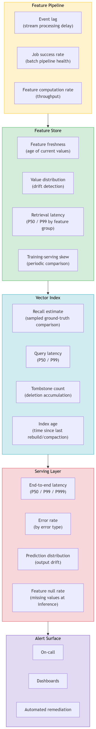
A few of these signals deserve particular attention because they’re routinely absent from production monitoring even in mature engineering organizations.
Feature null rate at inference time. When a feature value is missing — because an entity is new, because a pipeline failed, because a schema changed — most feature stores serve a default value silently. The null rate tells you how often this is happening. A sudden spike in null rate is a leading indicator of pipeline failure, schema drift, or cold start volume changes. Without tracking it, you’re flying blind on a significant dimension of input quality.
Prediction distribution drift. If the statistical distribution of your model’s outputs shifts — more extreme scores, a different mean, a collapsed variance — something upstream has changed. It might be a feature pipeline issue, a data quality problem, or genuine change in the underlying population. Monitoring output distribution doesn’t tell you which, but it tells you something changed, which is the signal that starts the investigation.
Training-serving skew over time. We covered training-serving skew as an architectural problem in Posts 2 and 3. Here it’s an operational metric. Periodically sampling serving-time feature values and comparing their distribution to training-time values catches skew that accumulates gradually — not from a single bad deployment, but from slow drift in source data, transformation logic, or serving behavior.
Failure Modes and Recovery Patterns
Pipeline Failures
Batch pipeline failures are the most straightforward: a job fails, the scheduler reports it, and the on-call engineer can rerun it. The question is whether the feature store degrades gracefully in the interim.
Design for stale-but-available. A feature store that returns stale values when the pipeline is delayed is better than one that returns errors. Stale values keep the model running, possibly with reduced quality. Errors stop the model from running entirely. Build explicit staleness thresholds: values older than N minutes trigger alerts; values older than M minutes trigger fallback behavior.
Streaming pipeline failures are more complex. A streaming job that falls behind on processing — accumulating lag in the event queue — may not fail outright. It may continue processing, but with increasing delay, silently delivering features that are progressively more stale. Stream lag monitoring is the signal: track the gap between when events are produced and when they’re processed, and alert when it crosses a threshold.
# Stream lag alert — conceptual
def check_stream_lag(consumer_group, max_lag_seconds):
    lag = kafka_consumer.get_lag(consumer_group)
    processing_rate = kafka_consumer.get_processing_rate(consumer_group)

    estimated_catchup_seconds = lag / processing_rate if processing_rate > 0 else float('inf')

    if estimated_catchup_seconds > max_lag_seconds:
        alert(
            f"Stream lag critical: {lag} messages behind, "
            f"estimated {estimated_catchup_seconds:.0f}s to catch up"
        )
Feature Store Failures
The online store is on the critical path for every inference request. Its failure mode is a total serving outage unless the system is designed with a fallback.
Fallback strategies in priority order:
- Serve from cache. If the serving layer caches recent feature retrievals, a brief online store outage can be absorbed without user impact for entities whose features were recently accessed.
- Serve defaults. Pre-computed default feature vectors — global averages, segment priors, or zero vectors — can keep the model running at reduced quality during an outage.
- Degrade gracefully. For some use cases, serving a simpler non-ML fallback (most popular items, rule-based decisions) is preferable to serving degraded ML predictions.
- Fail fast. For use cases where prediction quality is critical and degraded predictions are worse than no predictions, explicit failure with a clear error is the right answer.
The right strategy depends on your use case. What’s universally wrong is having no strategy — discovering during an incident that the serving layer has no fallback path and needs to be designed under pressure.
Vector Index Failures
Vector index failures are typically not binary. The index doesn’t go down — it degrades. Recall drops. Latency increases. Results become less relevant.
The operational response to index degradation depends on how it’s detected:
If recall drops below threshold: Trigger an index rebuild or compaction. In a segment-based architecture, compacting the most degraded segments may be sufficient. In a monolithic index, a full rebuild is required — which means managing traffic during the rebuild window.
If latency increases without load increase: Check tombstone accumulation. An index with a high fraction of deleted vectors will show latency increases before recall visibly degrades. Triggering a cleanup or rebuild early — before recall becomes a problem — is cheaper than reacting after the fact.
During an embedding model migration: The dual-index serving strategy is the safest path. Route queries to both the old and new index, returning results from the new index where available and falling back to the old index for records not yet recomputed. Monitor the migration percentage and recall on both indices throughout.
Capacity Planning: Designing Ahead of the Problem
Real-time AI systems fail at scale in predictable ways. Capacity planning is the practice of anticipating those failures before they occur.
Feature store capacity is driven by three variables: the number of entities, the number of features per entity, and the update rate. As any of these grow, both storage cost and write throughput requirements increase. The online store is typically the binding constraint — it’s expensive, and adding capacity requires planning time.
Model the growth of each variable separately. A user feature store that grows linearly with your user base is predictable. One that grows with user activity — where active users generate many feature updates per day — can grow superlinearly. Know which one you have.
Vector index capacity is driven by vector count, vector dimensionality, and query rate. Memory requirements for HNSW indices are roughly:
Memory (bytes) ≈ num_vectors × (dimension × 4 bytes + M × 8 bytes)

Where M is the HNSW connectivity parameter (typically 16-64)

Example: 10M vectors, 1536 dimensions, M=32
≈ 10M × (1536 × 4 + 32 × 8)
≈ 10M × (6144 + 256)
≈ 10M × 6400
≈ 64 GB
At 10 million vectors of typical embedding dimensionality, you’re looking at 50-100GB of memory just for the index — before accounting for the base vectors themselves. Planning for this before you hit the wall is significantly cheaper than scaling under pressure.
Inference compute capacity is the most familiar capacity planning domain, but AI workloads have spikier profiles than many web workloads. Model inference is CPU or GPU-bound, not I/O-bound, which means autoscaling has a longer warmup tail. Design for headroom that can absorb spikes without triggering cold start of new inference instances under load.
Incident Response: What to Do When It Breaks
When a real-time AI system degrades in production, the diagnosis path should be structured — not because engineers aren’t capable of reasoning under pressure, but because structured diagnosis is faster and less error-prone than ad hoc investigation.
A simple decision tree for real-time AI incidents:
Is end-to-end latency elevated?
├── YES → Check component latency breakdown
│         ├── Feature retrieval elevated? → Online store health
│         ├── Vector search elevated? → Index health (recall, tombstones)
│         └── Model inference elevated? → Compute resource saturation
│
└── NO → Is prediction quality degraded?
         ├── Is feature freshness stale? → Pipeline health (lag, job failures)
         ├── Is null rate elevated? → Schema change or cold start spike
         ├── Is output distribution shifted? → Feature distribution drift
         └── Is recall below threshold? → Index degradation
The key discipline is following the tree rather than jumping to conclusions. In complex systems, the symptom that’s most visible is often not the one that’s most actionable. A latency spike might be caused by vector search, or by feature retrieval, or by upstream traffic patterns that are saturating the online store. The monitoring signals tell you which — if they’re in place.
Runbooks — documented step-by-step procedures for common failure scenarios — dramatically reduce mean time to recovery. A runbook for “online store latency spike” that lists the specific metrics to check, the commands to run, and the escalation path removes the cognitive load of structuring the investigation under pressure. Writing runbooks before incidents is one of the highest-leverage operational investments a team can make.
The Operational Maturity Progression
Operational maturity for real-time AI systems isn’t a binary state. It develops in layers, and most teams are somewhere in the middle. A useful progression:
Level 0 — Reactive: The team discovers problems when users report them. No AI-specific monitoring. Recovery is ad hoc.
Level 1 — Instrumented: Basic metrics are in place for latency and availability. AI-specific signals (freshness, recall, distribution drift) are absent or manual.
Level 2 — Alerted: Alerts exist for the key AI-specific signals. On-call engineers are notified of degradation before users report it. Recovery is faster but still manual.
Level 3 — Documented: Runbooks exist for common failure scenarios. Incident response is structured and consistent. Post-mortems are conducted and drive improvements.
Level 4 — Automated: Common remediation actions are automated. Stream lag triggers automatic consumer group scaling. Index tombstone thresholds trigger automatic compaction. Freshness violations trigger automatic pipeline retries.
Most teams building real-time AI systems for the first time are at Level 0 or 1. Getting to Level 2 — instrumented and alerted on the AI-specific signals — is the single highest-leverage operational investment available. Levels 3 and 4 follow from the foundation that Level 2 provides.
Closing the Series
This series started with a simple observation: real-time AI systems that hum in development routinely hit problems in production, and those problems aren’t model problems — they’re infrastructure and operations problems.
The five posts have traced the full operational arc:
- Post 1: The gap between development and production, and the three categories of pressure that expose it
- Post 2: Feature pipelines — how to get features from raw events to a computed state with the freshness your model needs
- Post 3: Feature stores — the dual-store architecture, consistency enforcement, and the governance layer that makes reuse possible
- Post 4: Vector search — index degradation, recall monitoring, and hybrid filtering at scale
- Post 5: Operations — SLAs, latency budgets, the full observability stack, and the incident response patterns that reduce recovery time
The through-line is a shift in mindset: from thinking of the model as the system, to thinking of the pipeline as the system. At scale, the model is one component — a critical one, but one that depends entirely on the infrastructure surrounding it.
Building that infrastructure well — with explicit SLAs, comprehensive observability, thoughtful fallback strategies, and a documented path from alert to recovery — is what separates systems that scale from systems that struggle.
The problems are identifiable. The patterns are known. The investment pays for itself the first time a monitoring alert catches a degradation that would otherwise have reached your users.
Thanks for following along through this series. If you found it useful, the best thing you can do is share it with a teammate who’s building these systems for the first time — or forward it to someone who’s hitting these problems and doesn’t yet know why.
When Your AI Pipeline Grows Up Series
- Real Time AI at Scale
- Feature Freshness
- Feature Store
- Vector Search
- Operations – This Post!