
The Guardian: Human-in-the-Loop AI Governance
We’ve built a system that is Reliable and Affordable. Our Forensic Team is accurate, and The Accountant ensures we aren’t wasting our cognitive budget.
But in the enterprise, “capable” is not enough. For high-stakes decisions—like a $50k rare book audit or a compliance check—fully autonomous AI is a Liability.
Today, we introduce The Guardian: The final phase of our Production-Grade AI trilogy. We are implementing a standardized Human-in-the-Loop (HITL) checkpoint, moving from “Autonomous Agents” to “Augmented Intelligence.”
1. The Autonomous Trap: Confident Hallucination
In the first post of this series, The Judge proved that even the best models can confidently hallucinate. In a forensic audit, an agent might identify a water damage pattern and declare: “CRITICAL: High probability of modern forgery.” If that finding is wrong, the reputational and financial damage is severe. The problem isn’t the AI’s capability; it’s the lack of authorization. The agent is a worker, not a partner.
2. Implementing the “Governance Gate”
We need a way to “brake” the agent’s flow when it finds a high-severity issue. We’ve added the request_human_signature tool to our Forensic Analyzer MCP server project.
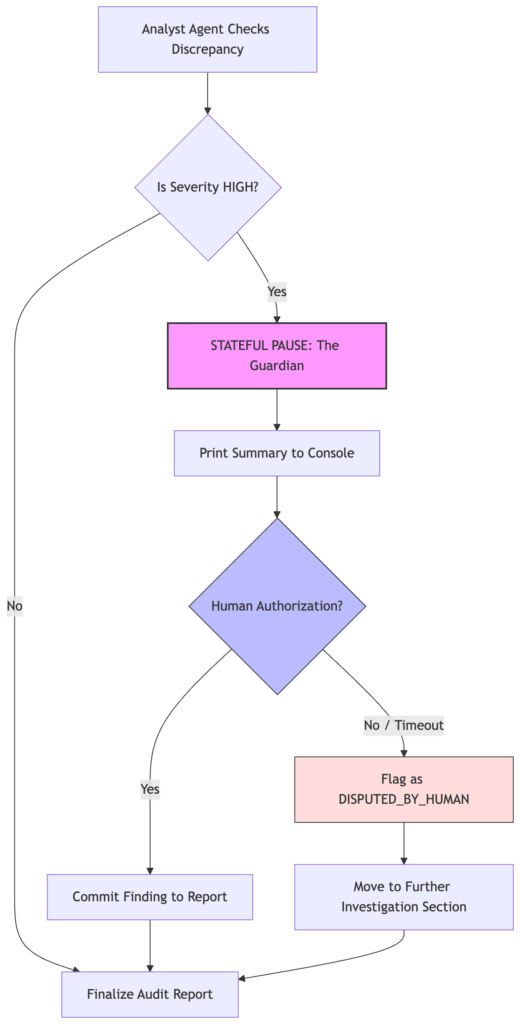
In orchestrator.py, we updated the logic. When the Analyst flags a “HIGH” severity discrepancy, the system performs a specialized handshake:
- Stateful Pause: The Python orchestrator interrupts the agent workflow.
- Authorization Prompt: It presents the evidence to the user via a CLI prompt.
- Cryptographic Signature: The user must authorize the finding before it’s committed to the final report.
# The Guardian's "Nuclear Key" moment in orchestrator.py
def _apply_guardian_handshake(analyst_result: dict) -> tuple[dict, list[dict]]:
    """
    Human-in-the-Loop: if Analyst has HIGH discrepancies, prompt for authorization.
    """
    disputed: list[dict] = []
    data = analyst_result.get("data") or {}
    disc = data.get("discrepancies", [])

    # Filter for the "High Stakes" findings
    high_disc = [d for d in disc if (d.get("severity") or "").upper() == "HIGH"]

    for d in high_disc:
        summary = f"[{d.get('severity')}] {d.get('field')}: {d.get('expected')} vs {d.get('observed')}"
        print(f"\n  Guardian: HIGH severity finding — {summary}")

        # THE STATEFUL PAUSE: The orchestrator stops and waits for a human
        answer = input("  Do you authorize this forensic finding? (yes/no): ").strip().lower()

        if answer != "yes":
            # Escalation: If not authorized, it's flagged as 'DISPUTED_BY_HUMAN'
            disputed.append({**d, "status": "DISPUTED_BY_HUMAN"})

    return analyst_result, disputed
By requiring a human to type ‘yes’, we are moving from Autonomous Assumption to Authorized Augmentation in the following ways:
- Severity-Based Intervention: “We don’t interrupt the user for every ‘Low’ or ‘Medium’ variance. We only trigger the Guardian for High-Severity findings—those that carry legal or financial liability. This preserves the ‘UX flow’ while maintaining safety.”
- The ‘Disputed’ State: “Notice that a ‘No’ from the human doesn’t just delete the finding. It moves it to a specialized ‘Requires Further Investigation’ section of the report. This ensures that the AI’s observation is preserved but clearly labeled as unauthorized.”
- Non-Interactive Fallback: “The code includes a check for EOFError (line 507). If the system is running in a non-interactive environment like a CI/CD pipeline, it defaults to ‘No’ (Dispute) for safety. Never default to ‘Yes’ for a high-risk authorization.”
3. Beyond the CLI: The Enterprise Handshake
This reference implementation uses a CLI input() prompt for simplicity. However, the MCP tool is standardized. In a production environment, this tool wouldn’t pause a Python script; it would:
- Trigger a Slack/Teams Alert to a senior auditor.
- Open a Jira Ticket for manual review.
- Request a Webauthn (Biometric) Signature in a web dashboard.
Summary: Building the Sovereign AI Stack
Across this series, we’ve moved from basic orchestration to a Production-Grade AI Mesh. We’ve proven that we can build systems that are:
1. Reliable: Audited by The Judge.
2. Sustainable: Optimized by The Accountant.
3. Safe: Governed by The Guardian.
The road to autonomous agents isn’t paved with more tokens; it’s paved with better guardrails.
What’s Next?
The code for the entire trilogy is available in the MCP Forensic Analyzer repository.
I’m currently working on Phase 3: The Sovereign Vault, where we will explore Local Multimodal Vision (processing artifact images without cloud egress) and PII Redaction to protect proprietary “Golden Data.”
Have questions about implementing these patterns in your own enterprise? Connect with me on LinkedIn or follow the blog for the next series.
The Production-Grade AI Series (Complete)
- Post 1: The Judge Agent: Who Audits the Auditors? (Reliability)
- Post 2: The Accountant: Cognitive Budgeting & Model Routing (Sustainability)
- Post 3: The Guardian: Human-in-the-Loop Governance (Safety)
Looking for the foundation? Check out my previous series: The Zero-Glue AI Mesh with MCP.