
Pattern Defined
Precise Definition: Hybrid Retrieval is an inference pattern that combines
semantic vector search with traditional keyword-based BM25 (Best Matching 25)
search, using a Reciprocal Rank Fusion (RRF) algorithm to produce a single,
unified result set.
Problem Being Solved
Vector search is excellent at “vibes” but terrible at “facts.” If you ask a
vector database for “Part #882-X,” it might return a document about “Part #881-Y”
because the semantic embedding of a part number is nearly identical to its
neighbor. This is the “Vector Hallucination” problem.
For a Director of Engineering, this creates a reliability gap. Your data needs a
map, not just a list. In the
Sovereign Vault,
where precise data retrieval is a prerequisite for high-integrity governance, a
“near miss” in retrieval is a total failure in compliance. As we saw in
Who Audits the Auditors?,
an agent can only be as reliable as the ground-truth data it can actually find.
Use Case
Consider our Vineyard Manager looking for a specific chemical application record
from 2024.
- Vector Search might pull records about “organic fertilizers” because the
“concept” is similar. - Keyword Search (BM25) will find the exact string “2024-FERT-08” but miss
the context of why it was applied.
By using Hybrid Retrieval, the system finds the exact document via keyword
matching while using semantic search to pull the surrounding context of the soil
conditions. The Manager gets the “map” of what happened, not just a list of
similar-sounding files.
Solution
The architecture requires a two-channel retrieval engine:
- Two-Channel Retrieval (Parallel):
- Dense Channel: Generate an embedding and search the vector index.
- Sparse Channel: Run a BM25 or full-text search against the same dataset.
- RRF (Reciprocal Rank Fusion): Apply a mathematical scoring system to
re-rank the results from both channels into a single, high-confidence list.
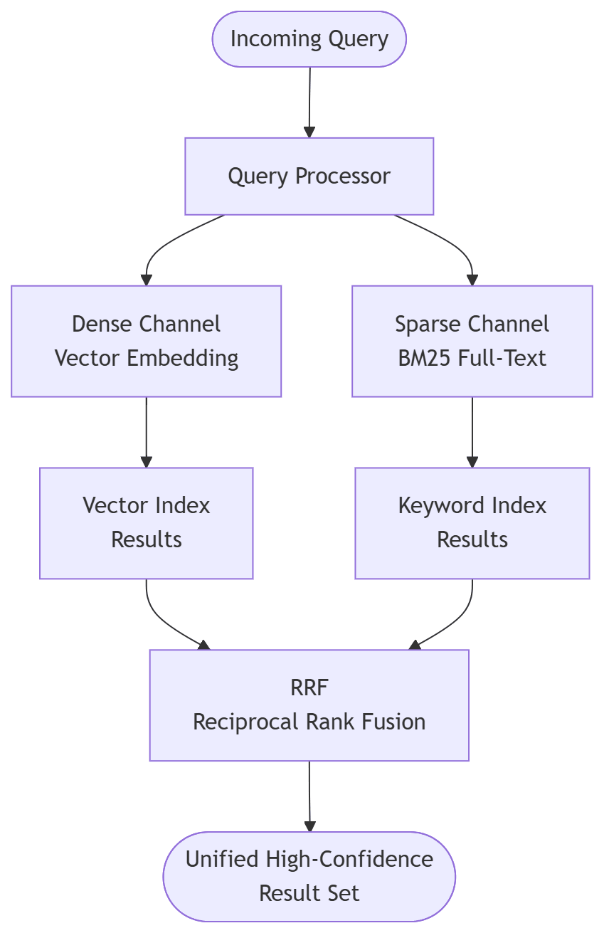
Two channels, one result: Dense and Sparse retrieval coverage at the RRF level.
In a FastAPI or Node.js environment using Meilisearch or Elasticsearch, this is often a
native feature that bridges your structured database with your unstructured AI
context.
Trade-Offs
The trade-off is Indexing Complexity vs. Precision. You are now maintaining
two types of indices for the same data, which increases your storage and
infrastructure footprint. While BM25 indices are lighter than vector indices, the
overhead in your ingestion pipeline is real.
For Technical Leaders, the cost is in the “Glue Code.” You must now manage
weightings—deciding if your system should trust the keyword or the vector channel
more for specific domains. This is another area where those two extra sprint cycles
of design are spent: tuning the balance between semantic intuition and keyword
precision.
Summary
Hybrid Retrieval ensures your AI isn’t just “guessing” at meaning. It provides
the literal anchor of keyword matching with the conceptual power of vector search.
Next Up
In two weeks, we move into the Agent Tool-Calling Pattern and build the “bandage” for the
most common break-point in agentic reliability.
Moving from Pattern to Production
The Sovereign Systems Specification will always remain entirely open-source and public. The community deserves a shared architectural vocabulary to fight the Prose Tax and secure local ingestion boundaries.
However, translating these conceptual primitives into hardened, concurrent enterprise infrastructure takes real engineering cycles. If you want to skip the trial-and-error and see these patterns in actual execution, I am opening early-access pre-orders for the Sovereign Systems Implementation Handbook.
While this public blog series explores what these patterns solve, the Handbook delivers the how, complete with:
– Production-Ready Blueprints: Fully implemented, modular code frameworks mapping out each pattern.
– Working Repositories: Production templates (FastAPI architectures) built for immediate deployment.
– Operational Playbooks: Line-by-line code walkthroughs, deployment topologies, and failure-mode checklists.
Secure your copy at the early-access price before the official launch.
Pre-Order the Sovereign Systems Implementation Handbook via Lemon Squeezy
Inference Pattern Series
- Inference Renaissance
- Speculative Decoding
- Context Compression Pattern
- Hybrid Retrieval – This Post
- Agent Tool-Calling – July 3
- The Sign-and-Sieve Pattern – July 17
- Multi-Model Routing – July 31
- Event-Driven Reflection Trigger – August 14