By now, the Backyard Quarry system has grown beyond its original intent.
We started with a pile of rocks.
We ended up with:
- a schema
- a capture process
- a processing pipeline
- storage and indexing
- digital representations of physical objects
Along the way, something interesting happened.
The problems stopped feeling unique.
Recognizing the Pattern
At first, the Quarry felt like a small, slightly absurd project.
But the more pieces came together, the more familiar it became.
The same structure appeared again and again:
- capture data from the physical world
- transform it into structured representations
- store it
- index it
- build systems on top of it
This isn’t a rock problem.
It’s a pattern.
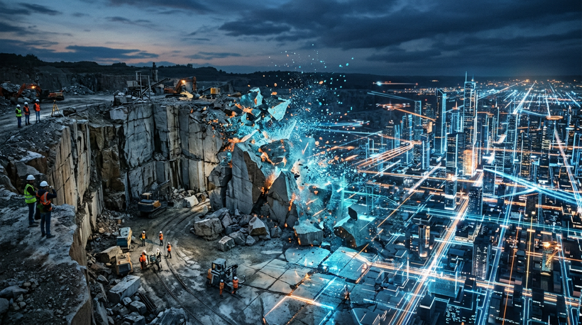
Where the Pattern Appears
Once you start looking for it, you see it everywhere.
Manufacturing Systems
Physical parts become digital records.
- components are tracked
- condition is monitored
- systems are modeled
Each part has a digital twin.
The system keeps everything connected.
Museums and Archives
Artifacts are cataloged and preserved.
- metadata describes objects
- images and scans capture detail
- provenance tracks history
The goal is the same:
Turn physical objects into structured, searchable systems.
Photogrammetry and 3D Capture
Entire environments can be captured and reconstructed.
- objects become meshes
- scenes become models
- real-world geometry becomes data
This is the Quarry pipeline, scaled up.
AI and Document Systems
Even text-based systems follow the same pattern.
- raw documents are ingested
- processed into structured formats
- indexed for retrieval
- used by applications
The inputs are different.
The structure is familiar.
Healthcare and Motion
Human movement becomes data.
- sensors capture motion
- signals are processed
- patterns are analyzed
- systems track change over time
This is where the idea of digital twins becomes more dynamic.
Not just objects.
But behavior.
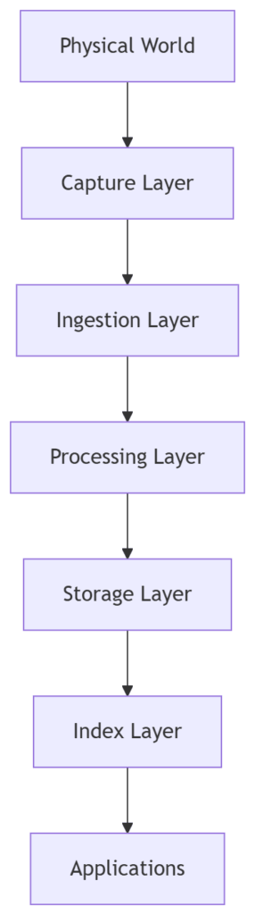
The Common Structure
Across all of these domains, the same core system emerges.
It doesn’t matter whether the input is:
- a rock
- a machine part
- an artifact
- a document
- a human movement pattern
The architecture is remarkably consistent.
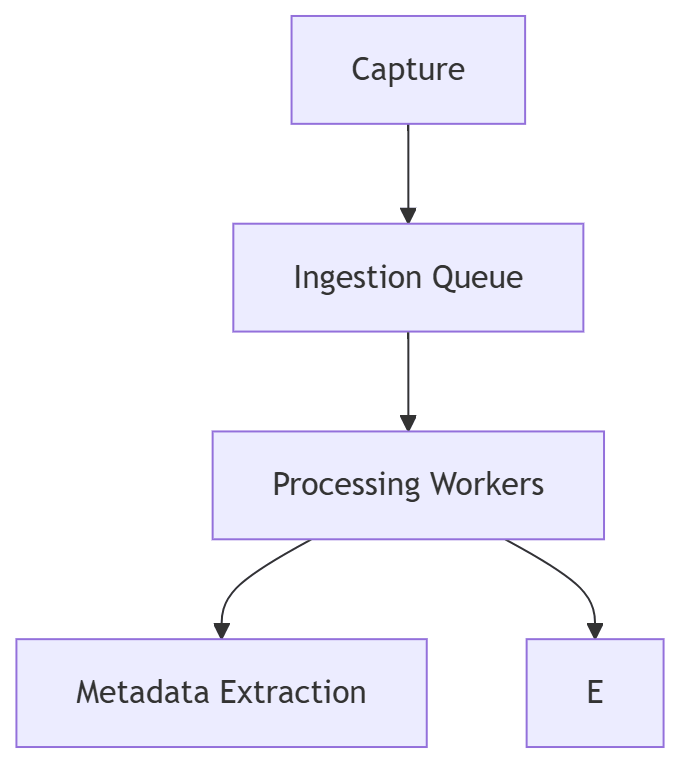
Capture.
Process.
Store.
Index.
Use.
The Value of Abstraction
One of the more useful realizations from the Quarry project is this:
The value isn’t in the specific object.
It’s in the system that handles it.
Once you understand the pattern, you can apply it in different contexts.
The details change.
The structure remains.
Systems, Not Features
At a certain point, it becomes less useful to think in terms of features.
Instead, the focus shifts to systems.
Questions change.
Instead of:
- How do we store this object?
- How do we search this dataset?
You start asking:
- How does data move through the system?
- Where are the bottlenecks?
- How do we handle growth?
- How do we handle imperfect inputs?
These are system-level questions.
The Real Takeaway
The Backyard Quarry started as a simple, somewhat comical, experiment.
But it revealed something broader.
Many modern systems are built on the same foundation:
- transforming real-world inputs into structured data
- building pipelines around that transformation
- enabling search, analysis, and interaction
The objects change.
The pattern doesn’t.
Looking Back
It’s a little surprising how far the idea traveled.
From:
- a pile of rocks
To:
- data modeling
- ingestion pipelines
- search systems
- digital twins
- scalable architectures
And now:
- recognizing patterns across industries
Not bad for something that started in the backyard.
What Comes Next
There’s one final step.
So far, we’ve explored:
- how to model objects
- how to capture them
- how to store and search them
- how systems scale
- how patterns repeat
In the final post, we’ll bring everything together.
A single view of the system.
A way to think about it as a whole.
Because once you can see the full structure, the pattern becomes difficult to miss.
And at that point, it becomes clear that the Quarry was never really about rocks.
It was about learning to recognize systems.
The Rock Quarry Series
- Turning Rocks into Data
- Designing a Schema for Physical Objects
- Capturing the Physical World
- Searching a Pile of Rocks
- Digital Twins for Physical Objects
- Scaling the Quarry
- Systems Beyond the Backyard – This Post
- From Rocks to Reality